Research Article
Volume 1 Issue 4 - 2017
Arrhythmia Detection from Photoplethysmography (PPG) Based on Pattern Analysis
1MSc Biostatistics- Faculty of Science, University of Hasselt, Belgium
2Professor, Director F02
3Senior Staff, Fibricheck
4Professor, Head of Bio-informatics, University of Hasselt, Belgium
2Professor, Director F02
3Senior Staff, Fibricheck
4Professor, Head of Bio-informatics, University of Hasselt, Belgium
*Corresponding Author: Dennis Boateng, MSc Biostatistics- Faculty of Science, University of Hasselt, Belgium.
Received: December 08, 2017; Published: December 15, 2017
Abstract
Introduction: In recent reports of the World Health Organization (WHO), three in ten deaths globally are caused by cardiovascular diseases from the heart and blood vessels that can cause heart attacks and strokes (W.H.O, 2014). Heart arrhythmia that presents in individuals can be useful indicators to Atria Fibrillation (AF) using traditional method of screening with Electrocardiogram (EKG). This gold standard of screening and detection is accurate however invasive, time consuming and expensive in comparison with nascent PPG technology implemented on smart devices for HRV measurements. The methods of PPG as an alternative to EKG requires accurate features since it is unclear which indicators of HRV are closely related to heart arrhythmia that can be used to quantify the severity. This report considers a live data obtained from Fibricheck with repeated measurement of 703 on 70 individuals between June 2016 to June 2017.
Objectives: The aim of the study was to create a classification methodology for the different arrhythmia's and evaluate the performance of this classifier based on a learning set and validation dataset and consequently create a probabilistic model that determines the chance of a specific arrhythmia to be classified into a specific category.
Methods: Features of HRV for both time domain and frequencies were derived and used for the fitting of classifiers and prediction models. Classification methods and algorithms are both found in Classification and Regression Trees (CART) and Random Forest (RF). Also methods of PCA were introduced to quantify the amount of information that is contained and explained by each feature explaining the variance covariance structure using a few linear combinations to reduce the effect of multi-collinearity.
Results: The conclusions drawn from the algorithms of CART and RF were comparable. An improved accuracy of overall features compared to the literature selected features was 0.94% with 95% CI: (0.907, 0.970) and 0.85% with 95% CI: (0.7926, 0.8894) respectively. The PCA corroborated the results obtained in RF and CART for the most plausible and biological feature related to AF as the mean and median since AF individuals tend to have a higher heart rate than normal individuals. The effects of further re-categorization strategy into two groups (normal-urgent) rather than three (normal-warning-urgent) im-proved the level of accuracy of 0.9786 with a 95% CI: (0.9508, 0.993). The prediction model obtained from the features generated and tested on the blinded data set did not miss-classify any warning individual as a normal patient.
Keywords: Photoplethysmography (PPG); World Health Organization (WHO); Heart Rate Variability (HRV); Atria Fibrillation (AF);
CART (Classi cation and Regression Trees)
Introduction
In recent reports of the World Health Organization (WHO), three in ten deaths globally are caused by cardiovascular diseases from the heart and blood vessels that can cause heart attacks and strokes (W.H.O, 2014). Cardiovascular diseases leading to premature deaths has high probability of successful prevention through a healthy diet, regular physical activity and avoiding the use of tobacco. The increasing levels of sophistication in lifestyle which includes our choice of foods and lack of regular exercises has sometimes led to undesired outcomes including mortality and morbidity (Bouwmeester., et al. 2009). The 21st century has made tremendous e orts in reducing or eradicating important communicable diseases in both developed and developing countries (Petersen, 2003) despite challenges in new infectious diseases that are present in certain populations.
This is due to the fact that more e orts were made in the development of diagnostic technologies, vaccine development and other therapeutic agents that prevented the onset of communicable diseases directly related to the environment. Despite these major breakthroughs in the combat against communicable diseases, non-communicable diseases which include cardiovascular diseases in contrast require more dedicated e orts in both technology for diagnosing, treatment and prevention (Alwan., et al. 2010; Beaglehole., et al. 2011; Ghaffar., et al. 2004).
Cardiovascular diseases con-tinue to be a challenge considering that the European Society of cardiology indicates that there are over six million cases of AF cases and the current burden in the western world is about two percent (Camm., et al. 2010) in comparison with the last decades and its prevalence is estimated to at least double in the next 50 years. In the African continent there exist many barriers and risk factors that contributes to Cardiovascular Diseases (CVD), however high blood pressure (or hypertension) is by far the commonest underlying risk factor for CVD (Cappuccio FP., et al. 2016). Recent reports indicate the steady rise of CVD mortality especially in low- and middle-income countries (LMICs) with rates of up to 300-600 deaths attributed to CVD per 100,000 population, and is projected to increase causing preventable loss of lives (Alwan A., et al. 2011). The consequences of the increasing trend especially in sub-Saharan Africa adds to the pressure on health facilities which have few resources and infrastructure in terms of health seeking for patients. Access to diagnostic services as well as medical professionals is di cult in relation to CVD.
Atria Fibrillation (AF) is directly linked to an increased risk of CVD or heart failure and co-morbidities in patients that present this condition (Camm., et al. 2010; Lloyd-Jones., et al. 2004). Serious AF may indicate damage to the myocardium, injuries to the pacemakers or conduction pathways and require immediate attention and remedies to sustain a patient and accounts generally for population prevalence of 0.4% to 1%, increasing with advancing age (Feinberg, Blackshear, Laupacis, Kronmal, & Hart, 1995; Fibrillation, 2001; Psaty., et al. 1997). Traditionally the gold standard used as a diagnostic instrument to measure the overall e ciency of the heart propagation and its electrical activities is called the Electrocardiogram. The device measures the various action potentials that the heart experiences for oxygenated blood to be carried away from the heart and de-oxygenated blood to carried back to the heart (Organization, 2014). The cycle of transmission and propagation begins with the heart natural pace maker that generates a signal across the right atrium inducing contraction and depolarization observed at various points indicated in figure 1. The various forms of irregularity can be determined easily by this overall electrical tracing of the heart by an EKG at each point or segment as the heart delivers its functions (Prasad & Sahambi, 2003).
Currently, innovative technologies implemented through smart phones Photoplethysmography (PPG) applications which is an optical technique that can be used to detect blood volume changes at the surface of the skin (Elgendi, 2012; Peng., et al. 2015; Tamura., et al. 2014) as an alternative to conventional EKG. The distance between two peaks in the EKG is also equivalent to that in a PPG by measurement of two peaks in terms of accuracy of measurements of breathing rate, cardiac RR intervals, and blood oxygen saturation (Scully., et al. 2012). In the context of health seeking, medical screening is a major step before any intervention is administered regarding the conditions of AF. Even recently diagnosed patients that show no signs of AF leading to no disease still require continuous screening to completely confirm their status more frequently than required of routine medical screening schedules. Heart related arrhythmia have different levels of severity and very often may be clouded with symptoms that are di cult to detect and classify leading to AF (Stevenson., et al. 2009; TORPPEDERSEN, KBER, Elming, & Burchart, 1997). The patterns revealed by nascent diagnostic technologies compared to the gold standard (EKG) are safe, cheap, and timely yet require extensive extraction of features that could indicate heart arrhythmia patients at risk. The PPG application requires the use of a smart phone as a platform and fortunately the penetration of smart phones in both Europe and Africa are comparable as they could benefit from these applications of PPG innovations.
The Poincare (Poincare plot) and Tachogram are well developed tools to analyse the RR sequences but there still exist other features that could be hidden from the RR peaks data extracted. It is unclear the various types of classifications that exist in PPG features that can be harnessed as an indicator for AF. It is valuable to harness all important classification features from PPG diagnostic techniques to help the GP make informed decisions. The ability of the PPG technology to capture such patterns is promising yet there are no single accepted measure of HRV despite its usefulness (Sabroe, Ellebk, & Qvist, 2016).
The context of classification procedures and appropriate algorithms should be biologically plausible to both the individual and the GP. Although sensors of current technologies for collecting PPG data are not clouded by subjectivity, they do not necessarily report a single, definitive depiction of reality hence the need to provide alternative approaches in analyzing and presenting relevant information embedded in the peaks of PPG applications with added features. The probabilities of making measurement errors and noise in data still remains a limitation factor of both hardware and software and cannot be completely ruled out in considering the most effective classification strategy. The classifier performance is based on learning data sets and evaluating its sensitivity and specificity of the PPG application. For particular cases, it will be important to distinguish the patterns that are of no danger and those that will need urgent decisions to be taken such as a surgery or even a medication as will be considered by GP
Methods
Basically, a light source and a detector are required to capture volumetrics in a PPG. The principle of light propagation is exploited in the vascular pulse as the wave of light travels in the body or tip of the finger. The exploration of the data using the peaks extracted should be the starting point to gain insight into the data prior to the classification and prediction analysis. A comprehensive idea about the data set enable one to put in context the classification procedures and appropriate algorithms that are biologically plausible to make inferences. The sequence of time intervals between the heartbeats is referred to as R-R intervals and this is measured over a period of anywhere from 10 min to 24h (Rompelman, O.,1982) this can also be basically translated in terms of BPM (Beats Per Minute).
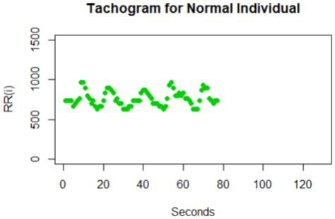
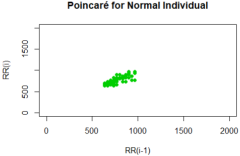
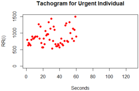
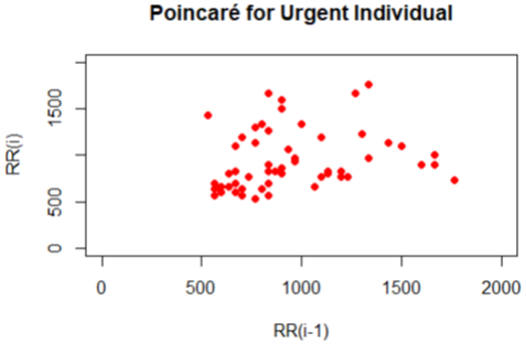
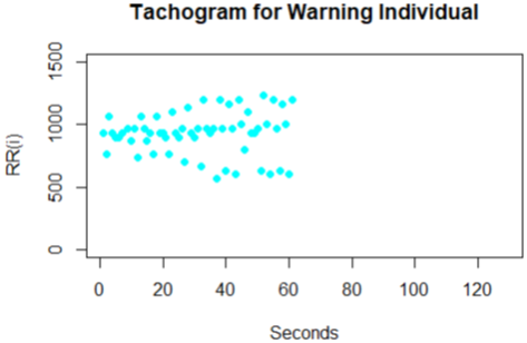
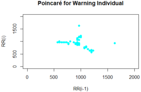
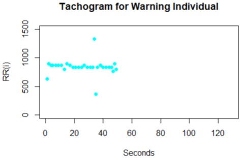
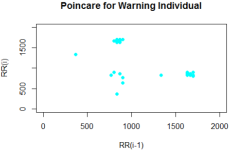
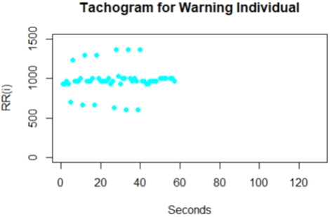
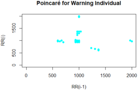
The Poincare plot is a scatter plot of the current R-R interval plotted against the preceding R-R interval which offers a quantitative visual technique as in figure 4,6,8,10 and 12 whereby the shape of the plot is categorized into functional classes (Woo, M. A ,1994; Woo, M. A,1992). An RR tachograph is a graph of the numerical value of the RR-interval (measured heartbeat-to-heartbeat) versus time also depicted in figure 3,5,7,9 and 11. In expressing of RR tachography, a Poincare plot which is a special case of a recurrence plot is a graph of RR(j) on the x-axis versus RR(j + 1) on the y-axis. The Poincare, Tachogram and box-plots were used to observe the variability over time.
The major limitation of the real life data obtained in PPG is encountered during recoding of the variables PPG do not directly indicate AF and an extensive manipulation of the data is required to generate both time and frequency HRV domain features which relate to the autonomic regulation. The desire to capture changes in the peak intensities is an important step prior to features generated, hence we look at peak intensities associated to R and call them J(i) and J(i+1) values which are consecutive for the generic feature functions. The intensity of the variation can be derived from the
JJ(i) = J(i+1)
J(i)
J(i)
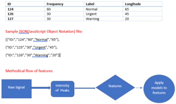
as well as BPM associated with RR(i) = R(i + 1) R(i). After this step we obtain the features based on these RR values and plug the features into our classifier. In our quest we derived and adapted 5 features as highlighted in table (1) as compliments which are well known in HRV inference. The data set used in this report is real life data obtained from Fibricheck company is embedded in a JSON le for each measurement taken of an individual HRV. The dataset consist of periodic measurement which may be repeated taken on 70 individuals. Some new variables or features were derived from statistical principles whiles others were also derived from literature studies conducted on HRV studies as in table (1) and these features are computed on the RR-values to be used for both classification and prediction.
Training and test data for model
The data will be split into two parts as the training data set to be used for fitting of classifiers and prediction models. To ensure that we have achieved satisfactory performance of the classifier, an independent validation dataset shall be used to cross validate our final model. Classification and Regression
The data will be split into two parts as the training data set to be used for fitting of classifiers and prediction models. To ensure that we have achieved satisfactory performance of the classifier, an independent validation dataset shall be used to cross validate our final model. Classification and Regression
Trees (CART) developed by Leo Breiman which is a decision tree algorithms implemented for classification or regression predictive modeling problems. A peculiar disadvantage associated with the CART is the problem of over fitting which sometimes can be resolved partly by pruning of the trees. CART are sensitive to changes in the data and sometimes results in an entirely different tree structure when very little adjustment is made.
| a | |
| Variable | Description |
| Minimum (Min) | Smallest observation from the individual sample data point |
| Maximum (Max) | Highest observation from the individual sample data point |
| Mean | The average of a set of each sample of the data point |
| Median | Central values of data points in which half are greater and less than itself |
| Standard Deviation (Std.Dev) | Measure of how much values vary from the mean given each data point |
| Correlation (Corr) | Indicates sufficiently strong relationship (direct or inverse) between subsequent data point |
| Skewness (Skew) | Measure of symmetry, or more precisely, the lack of symmetry in data point observed |
| kurtosis (Kurt) | Measure of whether the data are heavy-tailed or light-tailed relative to a normal distribution |
| Clusters (Clust) | Estimates the probable number of clusters in each Poincare plot of individual. The algorithm uses concepts of mixture models with an Expectation Maximization (EM) steps and selects clusters based on the Bayesian Information Criteria (BIC). |
| RMSSD (DSSB) | Expresses short term variability between samples using root of the mean squares of differences between adjacent Normal-Normal intervals |
| Turning Point Ratio (TPR) | Change in direction of the signals between consecutive peaks |
| PNN50 | Percentage of differences between adjacent Normal-Normal intervals that are greater than 50 ms; |
| Sample Entropy (SampEnt) | Measure to quantify the irregularity of a RR interval without bias |
| SDNN | Ratio of the mean to the standard deviations of Normal-Normal intervals |
Table 1: Variables derived from data.
a: The highlighted variables were derived and adopted from literature
a: The highlighted variables were derived and adopted from literature
Bagging and Random Forest
Bagging is to obtain an estimated average of the noise in the data by approximating the unbiased models that consequently reduces the variance (Friedman J., 2001). The disadvantages on over fitting and sensitivity in the CART is reconciled by bagging. This concept is implemented by considering a set of prediction in a regression context, where we t a model to the proposed training. Applying the method of bootstrap aggregation or bagging, an average of the prediction over a collection of bootstrap samples is obtained which reduces the variance. The disadvantage in the applicable use of bagging is in its size of correlation for the pairs of bagged trees which limits the benefits of averaging hence we introduce random forest as an alternative to the problem to improve the variance reduction of bagging. Variance reduction in RF is achieved by reducing the correlation between the trees, without increasing the variance by growing trees through a random selection of the input variables. Bagging refers to a special case of random forest where the number of parameters selected randomly to be used for the splitting nodes (m) = the total number of parameters used in the model.
Bagging is to obtain an estimated average of the noise in the data by approximating the unbiased models that consequently reduces the variance (Friedman J., 2001). The disadvantages on over fitting and sensitivity in the CART is reconciled by bagging. This concept is implemented by considering a set of prediction in a regression context, where we t a model to the proposed training. Applying the method of bootstrap aggregation or bagging, an average of the prediction over a collection of bootstrap samples is obtained which reduces the variance. The disadvantage in the applicable use of bagging is in its size of correlation for the pairs of bagged trees which limits the benefits of averaging hence we introduce random forest as an alternative to the problem to improve the variance reduction of bagging. Variance reduction in RF is achieved by reducing the correlation between the trees, without increasing the variance by growing trees through a random selection of the input variables. Bagging refers to a special case of random forest where the number of parameters selected randomly to be used for the splitting nodes (m) = the total number of parameters used in the model.
We basically grow trees on the bootstrap data randomly by selecting m<p (Friedman, J.,2001) subset of variables before the split and then when these trees are grown we now fit random forest regression predictor model to obtain a sample to be used for the bootstrap using the training data set. The principles of bootstrap is very beneficial to the random forest mechanism by recursively repeating steps for each terminal node of the tree, until the minimum node size nmin is acquired. An investigation for possible parameters could be tuned in the model to reduce the OOB errors. The known parameters that are used in the random forest estimation procedure includes; number of trees (ntree) to be grown for the prediction in the model which should not be very small number, to ensure that every input row gets predicted at least a few times as indicated in the manual of the Random Forest package in R. Also, the number of variables (mtry) that is randomly sampled for each candidate’s decision split was also used. Considering this two main variables with the default values for number of trees as 500 and mtry as the square root of number of parameters.
Classification and Prediction
The methods shall be used to explore the major classifications patterns for the heart arrhythmia that exist amongst individuals. The classification considered the accuracy of the individuals categorized in one of the three groups known as normal, urgent and warning groups respectively. The classification of the categories usually is the ability to discriminate suspected cases and non-suspected cases categories using the expected class-wise error rate. A blinded data set shall be used to evaluate the algorithms on accuracy and efficiency of the features to classify an individual. Initially RR sequences are obtained and this is used in both time domain and frequency features provided in table 1 for the fourteen features. A training model is built using different algorithms including random forest to identify features. The errors estimates for the OOB are tuned and best classifier is obtained using the test dataset.
The methods shall be used to explore the major classifications patterns for the heart arrhythmia that exist amongst individuals. The classification considered the accuracy of the individuals categorized in one of the three groups known as normal, urgent and warning groups respectively. The classification of the categories usually is the ability to discriminate suspected cases and non-suspected cases categories using the expected class-wise error rate. A blinded data set shall be used to evaluate the algorithms on accuracy and efficiency of the features to classify an individual. Initially RR sequences are obtained and this is used in both time domain and frequency features provided in table 1 for the fourteen features. A training model is built using different algorithms including random forest to identify features. The errors estimates for the OOB are tuned and best classifier is obtained using the test dataset.
Results
In this section, an initial exploration of the peaks was exploited from the JSON le. The peak intensities were extracted to reveal each individual data structure. A formal inquisition of the data structure was probed with the help of Tachograms, Poincare and box-plots. To enable us have a fair description of our visual impression we make use of the indicators normal, warning and urgent respectively. A random selection of individuals has been plotted side by side for both the Tachogram and Poincare plots for each particular individual.
Boxplots
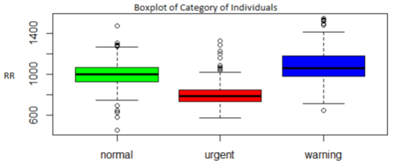
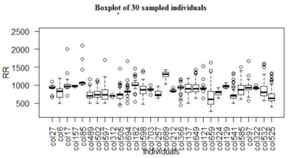
The box plot also offer an important depiction of standardizing the distribution of data based on each HRV measurement taken. Several features in the box plots of the sampled individuals indicate that we can consider the use of standard deviation, mean, minimum and maximum for each sample point. In figure 1, we observe that the high esteem means of the samples for the RR values in frequency standardization are recorded in the warning category. However the existence of outliers for the RR values were predominantly observed amongst the normal and urgent category of individuals. The skewness and kurtosis of the individual data points shown in figure 2 are clearly interesting features that were extracted from the box plot of random samples of individuals where the columns represents a particular individual.
The box plot also offer an important depiction of standardizing the distribution of data based on each HRV measurement taken. Several features in the box plots of the sampled individuals indicate that we can consider the use of standard deviation, mean, minimum and maximum for each sample point. In figure 1, we observe that the high esteem means of the samples for the RR values in frequency standardization are recorded in the warning category. However the existence of outliers for the RR values were predominantly observed amongst the normal and urgent category of individuals. The skewness and kurtosis of the individual data points shown in figure 2 are clearly interesting features that were extracted from the box plot of random samples of individuals where the columns represents a particular individual.
Tachogram and Poincare Theoretical Exploration for Indicators
Considered in this exploration there are many features that seems unique including the suggestions of clusters that are visible in the Poincare plots. The distribution of the individual peak intensities sequence was generated in a normal distribution of mixture modeling using an EM algorithm to estimate how many clusters are probable in each distribution or measurement. There were also features that seems indistinguishable considering the categorization of individuals into normal, urgent and warning.
Considered in this exploration there are many features that seems unique including the suggestions of clusters that are visible in the Poincare plots. The distribution of the individual peak intensities sequence was generated in a normal distribution of mixture modeling using an EM algorithm to estimate how many clusters are probable in each distribution or measurement. There were also features that seems indistinguishable considering the categorization of individuals into normal, urgent and warning.
The plots shown for the Tachogram and Poincare had the RR values standardized since the derived values are in samples and need appropriate conversion to frequencies for visualization. In figure 3 and 4 for the individual, the tachogram shows a serial correlation in the measurement with all points clustered in the Poincare plot at a specific location. Also in figure 5 and 6 for another individual taken, the tachogram has a stochastic behavior with its points all over the place. Furthermore, the tachogram figures in 7, 9 and 11 for the different individuals shows a combination of both serial correlation and stochastic characteristics.
The derived Poincare from each of the tachogram plots also have subtle differences yet unique in the region that spans the clusters. It is unclear in the plots produced by some warning individuals bearing resemblance to that of normal individuals even though some may be quite unique in certain cases. The uncertainty produced in these plots of a Poincare and Tachogram suggest further features to be obtained and used to investigate the strategy for discrimination category of individuals. Based on the Poincare plots we considered that a feature of clustering formation is present and can be used in the list of features.
Clusters from Poincare Plot
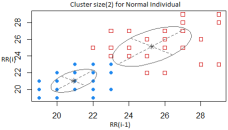
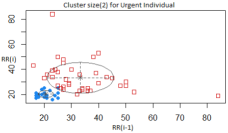
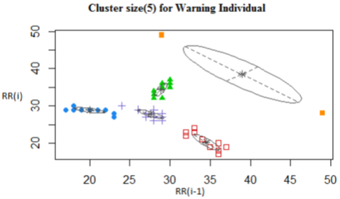
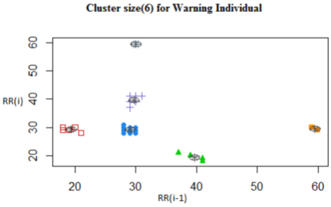
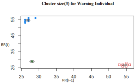
A random sample of individual Poincare plot suggested that the fixed number of G components could reasonably be estimated as a cluster between 1 and 10 clusters for each data point. The figures 13-17 shows the cluster sizes obtained from the Poincare plots of individuals for the three categories using the original sample of derived RR(i) as opposed to the standardized values in frequencies used for the Poincare and Tachogram plots. The values used on the x-axis in the cluster estimation is the RR(i-1) and that of the y-axis is the RR(i) as used in the Poincare plots. The ellipsoid in figure 13 for example shows the centroids as the mean vector for the normal individual with covariance matrix that determines the feature of the cluster.
A random sample of individual Poincare plot suggested that the fixed number of G components could reasonably be estimated as a cluster between 1 and 10 clusters for each data point. The figures 13-17 shows the cluster sizes obtained from the Poincare plots of individuals for the three categories using the original sample of derived RR(i) as opposed to the standardized values in frequencies used for the Poincare and Tachogram plots. The values used on the x-axis in the cluster estimation is the RR(i-1) and that of the y-axis is the RR(i) as used in the Poincare plots. The ellipsoid in figure 13 for example shows the centroids as the mean vector for the normal individual with covariance matrix that determines the feature of the cluster.
Although both figure 13 and 14 has a cluster size of 2 for the normal and urgent individuals respectively, they have unique centroids and eigen values characterizing their specific locations to estimate the feature of clusters. In the same regard figures 15-17 has different centroids for the mean vector. Also we adopted the concept that a cluster of size 1 was undefined and the threshold of 10 was reasonable as an estimate. In a publication of AF detection based on Poincare plot (Lian, J.,2011) implemented this strategy with the k-means algorithm. In our estimation of clusters the Mclust package implemented in R (Fraley, C.,2006) which estimates the number of clusters that best represents the sample of each individual data set and also the covariance structure of the spread points was used. This algorithm of Mclust used was also verified with that of the k-means and the results were consistent for each individual cluster estimated for an individual as in the k-means.
Basically the Mclust package makes a sweep over the number of clusters in each Poincare plot of an individual and applies BIC as a selection criterion. In Computer-assisted analysis of mixtures the C.A.MAN package provided by Bohning (Bohning D., et al. 1992) also applies the VEM (Vertex Expectation Maximization) algorithm with similar principles in implementation. The ease-of-use as well as the quick utilization of computing power motivated for the use of Mclust package from the large database of Fibricheck.
Model Selection and Fine-Tuning
The initial classification regression learner built from the training data set of the literature selected features has eight (8) terminal nodes and four (4) variables used. The variables selected were SDNN (Mean to the standard deviation), DSSB (RMSSD), PNN50, SampEnt (Sample Entropy). Also in the entire feature set there was nine nodes and seven features used which includes median, PNN50, SDNN, mini (minimum), Cluster, kurt (kurtosis), and Skew (skewness). Trees built was not pruned due to the fact that the cross validation error (X-val relative error) are already very near to the line indicative of good trimming.
The initial classification regression learner built from the training data set of the literature selected features has eight (8) terminal nodes and four (4) variables used. The variables selected were SDNN (Mean to the standard deviation), DSSB (RMSSD), PNN50, SampEnt (Sample Entropy). Also in the entire feature set there was nine nodes and seven features used which includes median, PNN50, SDNN, mini (minimum), Cluster, kurt (kurtosis), and Skew (skewness). Trees built was not pruned due to the fact that the cross validation error (X-val relative error) are already very near to the line indicative of good trimming.
Cross-Validation by Re sampling and CI Estimates
The computation of empirical estimates and CI on the OOB was carried out. The estimates of predictive accuracy was reported using the re substitution estimates. In random forest these estimates of predictive accuracy are referred to as out-of-bag error rates. A method of measuring the prediction error of the random forest which uses different bootstrap samples with replacement in making a decision. These estimates are generated on all features by running the random forest model several times for the prediction of error estimates using the test data. This repeated sequence each time generates estimates and CI that may be the same or sometimes have a subtle difference since the generation of OOB error rates are based on bootstrapping with replacement. It is worthwhile to loop over the estimates and CI to obtain robust empirical estimates. Hence both empirical estimate and Confidence Intervals are provided for the test and training repeatedly and consequently an accuracy of 0.94 with a 95% CI: (0.907, 0.970) indicates that the PPG test has 94.4% accuracy of classifying Individuals who are normal, warning or urgent on heart arrhythmia and this was a good indication of the PPG diagnostic capability.
The computation of empirical estimates and CI on the OOB was carried out. The estimates of predictive accuracy was reported using the re substitution estimates. In random forest these estimates of predictive accuracy are referred to as out-of-bag error rates. A method of measuring the prediction error of the random forest which uses different bootstrap samples with replacement in making a decision. These estimates are generated on all features by running the random forest model several times for the prediction of error estimates using the test data. This repeated sequence each time generates estimates and CI that may be the same or sometimes have a subtle difference since the generation of OOB error rates are based on bootstrapping with replacement. It is worthwhile to loop over the estimates and CI to obtain robust empirical estimates. Hence both empirical estimate and Confidence Intervals are provided for the test and training repeatedly and consequently an accuracy of 0.94 with a 95% CI: (0.907, 0.970) indicates that the PPG test has 94.4% accuracy of classifying Individuals who are normal, warning or urgent on heart arrhythmia and this was a good indication of the PPG diagnostic capability.
The results on the classification was repeated on the feature set that was adopted from literature and an accuracy using the empirical estimates was 0.846% with 95% CI: (0.7926, 0.8894). There was a slight decline in accuracy of about 10% difference in the limited feature set which had wide confidence intervals for accuracy. The second classification considers all the feature set (14) including 9 new features and 5 from literature. In both scenario the accuracy was judged and there was a better accuracy reported in the entire features (14) set compared to the 5 features set from literature.
The tuning of the hyper-parameters used in the random forest was also explored to obtain an improvement in accuracy. The default parameters used by the algorithm for RF hyper parameters for the number of trees as 500 and mtry as the square root of number of parameters, a training error of 5.98 initially was observed. After tuning the number of trees parameter (ntree = 300) as well as the number of features (parameters) to use for each split (mtry = 3), in the random forest model, the error rate in the training was improved to 5.77 after this adjustment by making several sweeps over the parameter space of the random forest hyper-features. The final model was adopted as there was a slight improvement after tuning the models and its associated parameters.
In both sensitivity considered for the two set of features, we observed that the sensitivity (Table 3a) remains high for the classification of individuals compared to the set of literature set that are reported in Table 3b. Also specificity is also high for this entire set of features and high in contrast to the feature set obtained from literature.
(a) Classification Outcome for combined (14) features (b) Classification Outcome for selected (5) features
| Prediction | Normal | Urgent | Warning | Class.Error | Normal | Urgent | Warning | Class.Error |
| Normal | 53 | 3 | 6 | 0.145 | 49 | 0 | 11 | 0.183 |
| Urgent | 0 | 79 | 3 | 0.036 | 1 | 75 | 11 | 0.138 |
| Warning | 3 | 1 | 86 | 0.044 | 11 | 3 | 72 | 0.163 |
Table 2: Outcomes of Classification for features.
(a) Validity Outcome for combined (14) features (b) Validity Outcome for selected (5) features
| Variable | Normal | Urgent | Warning | Normal | Urgent | Warning |
| Sensitivity | 0.9464 | 0.9518 | 0.9053 | 0.8033 | 0.9615 | 0.7660 |
| Specificity | 0.9494 | 0.9801 | 0.9712 | 0.9360 | 0.9226 | 0.8993 |
| Pos Pred Value | 0.8548 | 0.9634 | 0.9556 | 0.8167 | 0.8621 | 0.8372 |
| Neg Pred Value | 0.9826 | 0.9737 | 0.9375 | 0.9306 | 0.9795 | 0.8503 |
| Prevalence | 0.2393 | 0.3547 | 0.4060 | 0.2618 | 0.3348 | 0.4034 |
| Detection Rate | 0.2265 | 0.3376 | 0.3675 | 0.2103 | 0.3219 | 0.3090 |
| Detection Prevalence | 0.2650 | 0.3504 | 0.3846 | 0.2575 | 0.3734 | 0.3691 |
| Balanced Accuracy | 0.9479 | 0.9660 | 0.9382 | 0.8697 | 0.9421 | 0.8326 |
Table 3: Validity Outcomes for features predic.
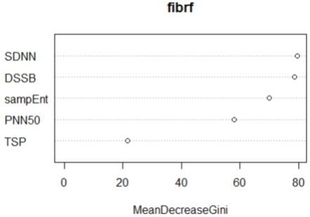
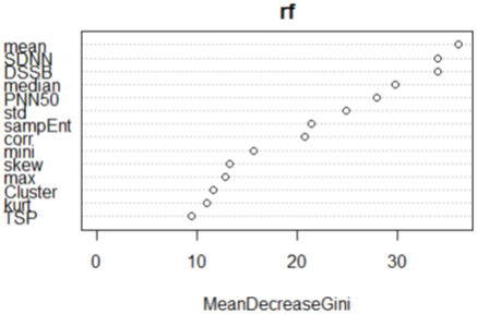
The relative importance for the set of predictors in a random forest is obtained through the Gini-index. The RF classification for the Gini-index was captured in the figures (18 & 19). A full description has been elaborated in Murthy., et al. (1994) and Su., et al. (2003) using this index. In the entire feature selection the best 3 features ranked by the random forest was the mean, PNN50 and SDNN (figure 19). However the best three features for the literature selected variables were SDNN, DSSB and sampleEntropy.
Validation Test on Blinded Dataset
In order to judge the methodology for reproducibility and reliability, the feature selection procedures was applied to a blinded dataset provided without indicators or labels of the individuals to be predicted. The motivation for such an added validation procedure is to ensure reliability of the OOB estimates which sometimes could be misleading in the random forest since they depend on a number of factors such as the number of observations, number of splits to be used.
In order to judge the methodology for reproducibility and reliability, the feature selection procedures was applied to a blinded dataset provided without indicators or labels of the individuals to be predicted. The motivation for such an added validation procedure is to ensure reliability of the OOB estimates which sometimes could be misleading in the random forest since they depend on a number of factors such as the number of observations, number of splits to be used.
Hence an external validation using a new dataset was used from Fibricheck and the algorithm was evaluated on its accuracy and reproducibility by repeating this new set of data as the test set. The original data set that had 703 samples was now considered for the calibration of a final model as the new training set to be used for the blinded dataset predictions which had 573 samples. The parameters used includes tuning the number of trees (ntree = 300) as well as the number of features (parameters) to use for each split (mtry = 3). All features were regenerated for the blinded dataset (14) and then a model fitted with random forest using the initial data was predicted.
The confusion matrix of this validation test set was provided by Fibricheck who had access to the original labels provided in the blinded data after the predictions were made for the category of heart arrhythmia an individual belongs.
The prediction ability was quite impressive since there was no individual who was labelled urgent predicted as normal individual. This means that we in practice could avoid missing individuals who had a slight possibility of a heart arrhythmia. The confusion matrix provided by fibricheck is reported in Table 4. The overall accuracy was 0.923%
| Prediction | Normal | Warning | Urgent | Class.Error |
| Normal | 413 | 9 | 1 | 0.024 |
| Warning | 12 | 59 | 8 | 0.253 |
| Urgent | 0 | 14 | 57 | 0.197 |
Table 4: Classification outcome for blinded data set.
Recategorization Strategy
The analysis was also reconsidered for the categorization schema for two groups instead of three to ascertain whether there could be a gain in the predictive measurements. After we had established that the entire set of features was adequate in predictive ability compared to the literature selected features, we proceeded with the two categorization schemes that is both warning and normal individuals were combined and considered normal category. The motivation was that in both the Poincare and Tachogram plots for the sampled individuals, there seemed much resemblance of pattern in the normal and warning groups. There was an indication of improvement in accuracy of this new classification with an accuracy of 0.9786 with a 95% CI: (0.9508, 0.993). Also measures of sensitivity and specificity were above 93% and there was no error in the prediction of the urgent groups after changing the categorization strategy used.
The analysis was also reconsidered for the categorization schema for two groups instead of three to ascertain whether there could be a gain in the predictive measurements. After we had established that the entire set of features was adequate in predictive ability compared to the literature selected features, we proceeded with the two categorization schemes that is both warning and normal individuals were combined and considered normal category. The motivation was that in both the Poincare and Tachogram plots for the sampled individuals, there seemed much resemblance of pattern in the normal and warning groups. There was an indication of improvement in accuracy of this new classification with an accuracy of 0.9786 with a 95% CI: (0.9508, 0.993). Also measures of sensitivity and specificity were above 93% and there was no error in the prediction of the urgent groups after changing the categorization strategy used.
In the feature selection using the Gini-index for the new categorization, the mean and median were among the top four features as reported earlier and quite consistent with the initial results obtained for all features considered using the initial categorization strategy.
(a) Initial Strategy using three category of outcomes (b) New categorization strategy using two outcomes
| Normal | Urgent | Warning | Normal + Warning | Urgent |
| 176 | 262 | 265 | 441 | 262 |
Table 5: Categorization frequencies.
| Variable | Normal |
| Sensitivity | 1.000 |
| Specificity | 0.933 |
| Pos Pred Value | 0.969 |
| Neg Pred Value | 1.000 |
| Prevalence | 0.679 |
| Detection Rate | 0.679 |
| Detection Prevalence | 0.701 |
| Balanced Accuracy | 0.967 |
(a) Validity Outcome for new category
| Normal | Urgent | Warning | |
| Prediction | normal | urgent | Class.Error |
| normal | 159 | 5 | 0.030 |
| urgent | 0 | 70 | 0.000 |
(b) Classification Outcome for new category
Table 6: Outcomes of New Strategy and prediction.
Principal Component Analysis
The hierarchical importance of features was further investigated using Principal Component Analysis (PCA). This is due to the fact that features that may be regarded as least important could have other features with overlapping information which is di cult to detect using the hierarchy of feature importance. PCA is concerned with explaining the variance covariance structure of a set of features through a few linear combinations of these features thereby reducing the effect of multi-collinearity issues. The main purpose for PCA is able to quantify the amount of information that is contained and explained by each feature. The importance of the features can be established without much doubts which play significant roles for PC since there seems to be slight incoherence in hierarchy of importance.
The hierarchical importance of features was further investigated using Principal Component Analysis (PCA). This is due to the fact that features that may be regarded as least important could have other features with overlapping information which is di cult to detect using the hierarchy of feature importance. PCA is concerned with explaining the variance covariance structure of a set of features through a few linear combinations of these features thereby reducing the effect of multi-collinearity issues. The main purpose for PCA is able to quantify the amount of information that is contained and explained by each feature. The importance of the features can be established without much doubts which play significant roles for PC since there seems to be slight incoherence in hierarchy of importance.
In an objective and simple methodology proposed to obtain a combination of predictors to explain the total variability, a criterion (Yeomans, K. A; 1982) on how the selection of components can be decided was used. This test criterion of predictors for the number of components is motivated by the eigen values of the components which have values greater than 1 are suitable candidates to used as the most optimal number of components. Furthermore, the eigen values shows that each component of P C5, P C8, ..., P C14 had eigen values less than 1. The eigen values of PC1, P C2,...,P C4, have values greater than one and hence plausible to be considered in explaining total variability in table 1. Hence, by considering these components not so much information will be lost, since the remaining PC explains only about 19% of the remaining variability.
The factor or component coefficients is also known as component loadings in PCA presented in table 7b. These correlation coefficients that exist between the variables indicated in the rows and factors indicated as columns. The principal component is the linear combination and loadings as a weight of all the fourteen original features, with mean feature contributing the highest as compared to the other features, while median is in the opposite direction with almost equal magnitude compared to the mean. The feature that contributed least to the first PCA is the corr with an opposite direction to the x-axis. The first principal component can be written as a linear combination of the features in the equation as follows:
PC1 = -9:109 (std) + 34:088 (mean) - 32:487 (median) - 10:106 (mini) - 12:781 (max) + 16:444 (skew) + 17:354 (kurt) - 7:384 (corr) + 23:222 (SDN N) - 7:854 (Clust) + 18:052 (DSSB) + 14:644 (T SP) + 18:274 (P N N50) + 12:418 (SampEnt)
This principal components linear combinations in table 13 with highest loadings has mean (34.088), median (-32.248), and SDNN (23.222) contributing significantly in P C1. These results are consistent with that obtained from RF where the Gini-index suggests that the four most important features includes the mean, SDNN, DSSB and median. In the second P C2 linear combinations, the median (-28.638) and max (-33.775) represent the most significant loading contributions. The median remains consistent while the max with such high loading contributions was unexpected as the RF suggested it was amongst the lowest ranked feature of importance. Also the sampEnt (22.344) contributed most significantly in terms of loading for P C3 however this was not the effect of importance connoted by the RF for the same feature in the hierarchy of importance. This results for P C1 linear combinations that coincides with the RF connotes that these features are most important to be considered if we were to reduce the number of features without losing much efficiency.
| Features | Eigen.Values | %Variance | Cum.Variance |
| PC1 | 4.66 | 33.30 | 33.30 |
| PC2 | 3.73 | 26.62 | 59.91 |
| PC3 | 1.91 | 13.66 | 73.57 |
| PC4 | 1.04 | 7.44 | 81.01 |
| PC5 | 0.95 | 6.82 | 87.83 |
| PC6 | 0.73 | 5.18 | 93.01 |
| PC7 | 0.43 | 3.06 | 96.07 |
| PC8 | 0.25 | 1.81 | 97.88 |
| PC9 | 0.11 | 0.76 | 98.65 |
| PC10 | 0.10 | 0.74 | 99.39 |
| PC11 | 0.04 | 0.30 | 99.68 |
| PC12 | 0.02 | 0.17 | 99.85 |
| PC13 | 0.02 | 0.11 | 99.96 |
| PC14 | 0.01 | 0.04 | 100.00 |
(a) Eigen values of the covariance matrix
| PC1 | PC2 | PC3 | PC4 | |
| std | -9.109 | 5.579 | 7.446 | 1.383 |
| mean | 34.088 | -0.514 | -8.75 | -0.252 |
| median | -32.487 | -28.638 | -8.432 | -0.181 |
| mini | -10.106 | -18.211 | 1.295 | 1.101 |
| max | -12.781 | -33.775 | -4.579 | 6.268 |
| skew | 16.444 | 2.723 | -4.03 | -1.102 |
| kurt | 17.354 | -14.571 | 1.65 | 1.936 |
| corr | -7.384 | 4.421 | -2.094 | 0.48 |
| SDNN | 23.222 | -1.396 | 7.651 | -2.798 |
| DSSB | 18.052 | 1.941 | -4.009 | 0.5 |
| TSP | 14.644 | -10.092 | 9.456 | -0.64 |
| PNN50 | 18.274 | -1.837 | 15.35 | -3.772 |
| SampEnt | 12.418 | -1.59 | 22.344 | -4.837 |
| Clust | -7.854 | -12.668 | -4.425 | 1.628 |
(b) Coefficients of PCA
Table 7: Principal Component of features.
Discussion
Prior to the features generation and selection, there was a careful pre-processing of the peaks which was key to developing a successful classification procedure. Due to this fact the raw data from PPG peaks should be the starting point for any relevant methodology to be implemented since disregard for this could lead to spurious interpretations.
There was generally a good indication of sensitivity and specificity of PPG in the study population as the tests discriminated those individuals with and without AF. This was evident and quite spectacular that the predictions made on the blinded data did not misclassify individuals who had an urgent condition of heart arrhythmia as normal when the confusion matrix was obtained from fibiricheck. In the face of the evidence provided this reaffirms our confidence in the methodology for features derived and possible actions and guidelines for individuals decision on their health as well as policies to use PPG as a front line to screen for suspected cases of arrhythmia.
Furthermore, investigations for the new classification compared with the original classification used in the study presented improved estimates of accuracy, sensitivity and specificity. The new classification seems more natural for distinguishing individuals who are cases and those who are not. However the adoption of this new classification with improved estimates of accuracy, sensitivity and specificity is more appealing since the W.H.O recommendations for diagnostic instruments places a priority/preference towards instruments with higher sensitivity and specificity. This is to ensure that the treatment assigned pending the evidence provided by the PPG diagnostic must clearly rule out any clinical consequences associated with treating potentially false positive and negative test since its consequence may outweigh the potential cost-saving benefits. The results can also be viewed and interpreted by individuals of the application as a form of risk assessment to their health status even though they may be yet asymptomatic in consultation with their health practitioners. The accuracy on the new categorization is quite impressive hence individuals who are predicted as urgent could consider they are at higher risk compared to individuals predicted as normal.
In this regard AF obtained from the diagnostic using the PPG is very important in the early detection and prevention of strokes considering the accuracy of 97% in comparison to the high costs or invasive procedures of EKG. In certain geographical locations where infrastructure and maintenance for the EKG are not available, the PPG could be used as a substitute due to its high predictive ability. A particular benefit that could be derived from the extensive use of smart phones with PPG application in Europe and particular reference to Africa is its simplicity to diagnosis AF with high accuracy compared to the traditional method using EKG. Considering the 10-20 million suspected hypertension cases in sub-Saharan Africa, it is estimated that 250,000 deaths could be averted annually if adequate diagnosis and appropriate treatment are administered (Cooper, R. S., 1998). The limitations associated with EKG-based strategies prompts alternative diagnostic methods such as PPG to compliment the diagnostics of AF which is di cult to diagnose. The limitations of the EKG includes short monitoring period (24-h Holter EKG), as well as requiring patients to trigger the recorder (the patient-triggered event recorder).
The classification and prediction from the random forest for the entire 14 features had three top most important variables as mean, SDNN (Mean to the Standard deviation) and RMSSD after the model was tuned. These features selected in our results were comparable to recent studies conducted by Shun-Chun
(Tang, S. C., 2017) which used a logistic regression analysis and revealed similar independent PPG features including three pulse interval (PIN)-related (mean, mean of standard deviation, and sample entropy). In our case the simple method of trees also suggested the median and mean of standard deviation as two key features out of the seven features selected by the tree.
The main difference encountered in applying a PCA is for dimensionality reduction of the features available while random forest could use the set of reduced set to make classification or prediction. Our finding in the PCA corroborates the mean feature as the most strongly correlated component to P C1 as suggested by the random forest Gini-index ranking of features. Also findings from PC1 and PC2 reveal the median as one of the most influential contributors to the components as suggested by RF and CART independently. In a biological perspective, the mean and median measurement of the pulse interval are very prominent features to AF as the results of CART, RF and PCA con rms. It is quite logical to interpret this finding that individuals with Atria Fibrillation tends to have a higher heart rate than normal or warning individuals.
Conclusion and Recommendation
The PPG is a good diagnostic instrument for the diagnosing of heart Arrhythmia in individuals. The comparative advantage of the innovative diagnostic is more feasible and cost-effective for the detection of AF. In the hierarchy of diagnostic tests, this should be considered as the first line by medical practitioners before any complicated and expensive tests/diagnosis are required for the individual. PPG as a diagnostic technology for AF in the Belgian sampled population is a good tool that will augment the screening of patients to decrease the prevalence of AF by targeting those who need treatment most. The PPG ap-plication should be encouraged and recommended to peripheral public health facilities without trained cardiologist staff and technicians as well as non equipped infrastructure to correctly identify, monitor and complement AF diagnosis where there is high prevalence in the population.
Further studies will need to be conducted to access the relationship between AF and demographic characteristics which includes the location, age and gender of individuals. This is because AF is linked closely to co morbidities and its associated patient characteristics. A confirmation of these results can be an added benefit in the prediction and classification strategy.
References
- Alwan A., et al. “Monitoring and surveillance of chronic non-communicable diseases: progress and capacity in high-burden countries”. The Lancet 376.9755 (2010): 1861-1868.
- Ball J., et al. “Atrial fibrillation: profile and burden of an evolving epidemic in the 21st century”. International journal of cardiology 167.5 (2013): 1807-1824.
- Beaglehole R., et al. “Priority actions for the non-communicable disease crisis”. The Lancet 377.9775 (2011): 1438-1447.
- Boden-Albala B., et al. “Lifestyle factors and stroke risk: exercise, alcohol, diet, obesity, smoking, drug use, and stress”. Current Atherosclerosis Reports 2.2 (2000): 160-166.
- Bouwmeester H., et al. “Review of health safety aspects of nanotechnologies in food production”. Regulatory Toxicology and Pharmacology 53.1 (2009): 52-62.
- Camm AJ., et al. “Corrigendum to: Guidelines for the management of atrial fibrillation”. European Heart Journal 31 (2010): 2369-2429.
- Cooper HA., et al. “Light-to-moderate alcohol consumption and prognosis in patients with left ventricular systolic dysfunction”. Journal of the American College of Cardiology 35.7 (2000): 1753-1759.
- Elgendi M. “On the analysis of fingertip photoplethysmogram signals”. Current Cardiology Reviews 8.1 (2012): 14-25.
- Feinberg WM., et al. “Prevalence, age distribution, and gender of patients with atrial _brillation: analysis and implications”. Archives of Internal Medicine 155.5 (1995): 469-473.
- Go AS., et al. “Prevalence of diagnosed atrial fibrillation in adults: national implications for rhythm management and stroke prevention: the AnTicoagulation and Risk Factors in Atrial Fibrillation (ATRIA) Study”. JAMA285.18 (2001): 2370-2375.
- Furberg CD., et al. “Prevalence of atrial fibrillation in elderly subjects (the Cardiovascular Health Study)”. The American Journal of Cardiology 74.3 (1994): 236-241.
- Ghaffar A., et al. “Burden of non-communicable diseases in South Asia”. BMJ: British Medical Journal 328.7443 (2004): 807-810.
- Gray G., et al. “Medical Screening of Subjects for Acceleration and Positive Pressure Breathing La Surveillance Medicale des Sujets Relative aux Accelerations et a la Surpression Ventilatoire (No. AGARD-AR-352)”. Advisory group for aerospace research and development NEUILLY-SUR-SEINE (France) (1997):
- Heemstra HE., et al. “The burden of atrial fibrillation in the Netherlands”. Netherlands Heart Journal 19.9 (2011): 373-378.
- WHO MONICA Project Principal Investigators. “The World Health Organization MONICA Project (monitoring trends and determinants in cardiovascular disease): a major international collaboration”. Journal of clinical epidemiology 41.2 (1988): 105-114.
- Kannel WB., et al. “Current perceptions of the epidemiology of atrial fibrillation”. Cardiology clinics 27.1 (2009): 13-24.
- Krijthe BP., et al. “Projections on the number of individuals with atrial fibrillation in the European Union, from 2000 to 2060”. European heart journal34.35 (2013): 2746-2751.
- Lloyd-Jones DM., et al. “Lifetime risk for development of atrial fibrillation”. Circulation 110.9 (2004): 1042-1046.
- World Health Organization. “Management of Substance Abuse Unit”. Global status report on alcohol and health (2014):
- Peng RC., et al. “Extraction of heart rate variability from smartphone photoplethysmograms”. Computational and mathematical methods in medicine (2015):
- Petersen PE. “The World Oral Health Report 2003: continuous improvement of oral health in the 21st centurythe approach of the WHO Global Oral Health Programme”. Community Dentistry and oral epidemiology 31.s1 (2003): 3-24.
- Prasad GK., et al. “Classification of ECG arrhythmias using multi-resolution analysis and neural networks”. Conference on Convergent Technologies for the Asia-Pacific Region 1 (2003): 227-231.
- Psaty BM., et al. “Incidence of and risk factors for atrial fibrillation in older adults”. Circulation 96.7 (1997): 2455-2461.
- Ruo B., et al. “Racial variation in the prevalence of atrial fibrillation among patients with heart failure: the Epidemiology, Practice, Outcomes, and Costs of Heart Failure (EPOCH) study”. Journal of the American College of Cardiology 43.3 (2004): 429-435.
- Sabroe JE., et al. “Intraabdominal microdialysis-methodological challenges”. Scandinavian Journal of Clinical and Laboratory Investigation 76.8 (2016): 671-677.
- Scully CG., et al. “Physiological parameter monitoring from optical recordings with a mobile phone”. IEEE Transactions on Biomedical Engineering 59.2 (2012): 303-306.
- Stevenson LW., et al. “INTERMACS profiles of advanced heart failure: the current picture”. The Journal of Heart and Lung Transplantation 28.6 (2009): 535-541.
- Tamura T., et al. “Wearable photoplethysmographic Sensors-past and present”. Electronics 3.2 (2014): 282-302.
- TORPPEDERSEN., et al. Classification of sudden and arrhythmic death”. Pacing and clinical electrophysiology 20.10 (1997): 2545-2552.
- World Health Organization. “10 facts on the state of global health” (2014):
- Zoni-Berisso., et al. “Epidemiology of atrial fibrillation: European perspective”. Clinical Epidemiology 6 (2014): 213-220.
- Rompelman O., et al. “The measurement of heart rate variability spectra with the help of a personal computer”. IEEE Transactions on Biomedical Engineering 7 (1982): 503-510.
- Woo., et al. “Complex heart rate variability and serum norepinephrine levels in patients with advanced heart failure”. Journal of the American College of Cardiology 23.3 (1994): 565-569.
- Woo MA., et al. “Patterns of beat-to-beat heart rate variability in advanced heart failure”. American heart journal 123.3 (1992): 704-710.
- Friedman J., et al. “The elements of statistical learning”. Springer series in statistics 1 (2001):
- Tang SC., et al. “Identification of Atrial Fibrillation by Quantitative Analyses of Fingertip Photo- plethysmogram” Scientific Reports 7 (2017):
- Peel D., et al. “Robust mixture modelling using the t distribution”. Statistics and computing 10.4 (2000): 339-348.
- Dempster AP., et al. “Maximum likelihood from incomplete data via the EM algorithm”. Journal of the royal statistical society. Series B (methodological) (1977): 1-38.
- Fraley C., et al. “MCLUST version 3: an R package for normal mixture modeling and model-based clustering”. WASHINGTON UNIV SEATTLE DEPT OF STATISTICS (2006):
- Celebi ME. “Partitional clustering algorithms”. Switzerland: Springer (2015):
- Kaufman L., et al. “Finding groups in data: an introduction to cluster analysis”. John Wiley & Sons (2009): 344.
- Lian J., et al. “A simple method to detect atrial fibrillation using RR intervals”. The American journal of cardiology 107.10 (2011): 1494-1497.
- Yeomans KA., et al. “The Guttman-Kaiser criterion as a predictor of the number of common factors”. The Statistician (1982): 221-229.
- Bohning D., et al. “Computer-assisted analysis of mixtures (CA MAN): statistical algorithms”. Biometrics (1992): 283-303.
- Cappuccio FP., et al. “Cardiovascular disease and hypertension in sub-Saharan Africa: burden, risk and interventions”. Internal and Emergency Medicine 11.3 (2016): 299-305.
Citation:
Dennis Boateng., et al. “Arrhythmia Detection from Photoplethysmography (PPG) Based on Pattern Analysis”. Therapeutic
Advances in Cardiology 1.4 (2017): 165-183.
Copyright: © 2017 Dennis Boateng., et al. This is an open-access article distributed under the terms of the Creative Commons Attribution License, which permits unrestricted use, distribution, and reproduction in any medium, provided the original author and source are credited.





 Scientia Ricerca is licensed and content of this site is available under a Creative Commons Attribution 4.0 International License.